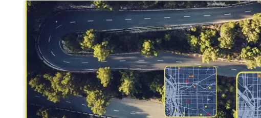
Atypical Curves Last update : 2024-02-06 Publisher Michelin Mobility Intelligence Scope France Identify the risk profile of curves to anticipate the works to be done before accidents happen.
Crash Probability Hotspots Last update : 2024-02-06 Publisher Michelin Mobility Intelligence Scope USA Identify and rank, by crash probability indicator, hotspots within your road network.
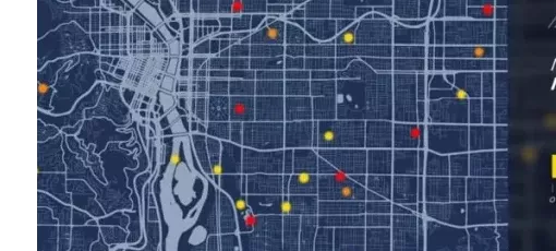
Detailled driving events Last update : 2024-02-06 Publisher Michelin Mobility Intelligence Scope USA, France Get detailed information on driving events within your road network.
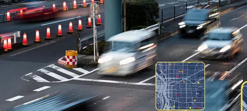
Driving Events Last update : 2024-02-06 Publisher Michelin Mobility Intelligence Scope USA, France Detect, locate, and count driving events within your road network.
Driving Events at Intersection Last update : 2023-07-20 Publisher Michelin Mobility Intelligence Scope USA Detect, locate, and count driving events within and around intersections within your road network.
Excessive Speeding Last update : 2023-07-20 Publisher Michelin Mobility Intelligence Scope USA Detect, locate and count excessive speeding driving events within your road network.
Harsh Acceleration Last update : 2023-07-20 Publisher Michelin Mobility Intelligence Scope USA, France Detect, locate and count harsh acceleration driving events within your road network.
Harsh Braking Last update : 2023-07-20 Publisher Michelin Mobility Intelligence Scope USA, France Detect, locate and count harsh braking driving events within your road network.
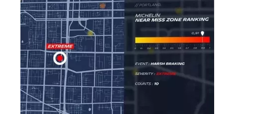
Near Miss Hotspots: Severity Ranking Last update : 2024-01-10 Publisher Michelin Mobility Intelligence Scope USA Locate, assess and rank by severity near miss hotspots within your road network.
Phone Handling Last update : 2023-07-20 Publisher Michelin Mobility Intelligence Scope USA Detect, locate and count phone handling events within your road network.
Speeding hotspots Last update : 2023-07-20 Publisher Michelin Mobility Intelligence Scope France Detect and locate above the speeding limit driving behaviours within your road network.
Suspected Collisions Last update : 2023-07-20 Publisher Michelin Mobility Intelligence Scope USA Detect, locate and count suspected collisions events within your road network.